Solea™ Operation Manual SOTIRIA Technology · Version 260220
1. Manufacturer Instructions and Safety Notes
- The device is intended for underwater operation.
- After each deployment, clean the device and its cable with fresh water and mild dish soap. During long deployments, retrieve and repeat cleaning at least once a month.
- Store in a dry environment at room temperature, away from children and flammable materials.
- Do not place the device near strong magnetic fields.
- For optimal operation, do not place near ferromagnetic objects (e.g. steel frames, anchor chains).
- Recommended submersion depth: up to 50 m. Do not submerge beyond 300 m or in corrosive liquids.
- Do not expose to fire or temperatures higher than recommended.
- Do not open the device or modify its hardware or software.
- Do not impact, puncture, or heat the device.
- Do not bend, press or scratch the hydrophone.
- The hydrophone includes an exposed wire connected to device Ground. Do not apply any voltage to this wire.
- For best hydrophone sensitivity, use it when fully submerged.
- Do not connect the device wires to voltages different from those specified in this manual.
- Do not power outside the range of 7–30 VDC.
- Do not extend the cable or use cable with different specifications.
- Do not pull the device from its cable. Avoid bending or twisting it.
- Keep the device as stationary as possible during operation, to avoid motion artifacts. The use of a non-ferromagnetic mounting frame is recommended.
- To prevent galvanic corrosion, avoid direct contact of the aluminum enclosure with other metals.
⚠ CAUTION: The device includes a pressure relief valve. Tighten it clockwise by hand before deployment. Otherwise, the device will be flooded and permanently destroyed.
ℹ NOTE: The device includes a resettable (PPTC) fuse. After a short circuit, wait up to 10 minutes before retrying to operate the device.
2. Device Description
The device includes a magnetic sensor, an acoustic sensor, an Inertial Measurement Unit (IMU) and an environmental sensor (temperature/humidity/pressure), as well as the necessary electronics for edge processing. It can be powered by a 7–30 VDC, ≥1 A power supply and communicates via RS-485 using Modbus RTU registers. Alternatively, a power and communication device (sold separately) can be used to retrieve data via Wi-Fi, 4G, Ethernet, or USB.
2.1 Magnetic Sensor
- 3-axis open-loop fluxgate sensor for detecting slow (DC – 10 Hz) magnetic field variations
- Measures magnetic field in each axis (X, Y, Z) in nT
- Outputs the results, as well as the Total magnetic field magnitude, i.e. √(X² + Y² + Z²) and the deviation of the latest reading from a rolling-mean baseline over the recent samples
- The deviation output is generally the most useful result, as it highlights sudden magnetic field anomalies, unaffected by slow geomagnetic field changes or long-term magnetic drift
- Optional per-axis temperature compensation (βx, βy, βz in nT/°C, with reference temperature T0) can be applied to the decimated stream — see §4.3 for the register map and the dashboard Temperature Compensation card for entering coefficients. Disabled by default; coefficients are derived per deployment from a regression of
x_dec/y_dec/z_decagainst the on-board temperature on a quiet window
2.2 Acoustic Sensor
- PZT-based hydrophone
- Captures and processes audio data
- Outputs top 10 dominant frequencies (FFT) with Sound Pressure Levels (SPL) in dB re 1 μPa
2.3 IMU (Inertial Measurement Unit)
- Accelerometer/gyroscope/magnetometer combination
- Captures device orientation in 3D space
- Outputs yaw, pitch, and roll in degrees
2.4 Environmental Sensor
- Temperature, humidity, and pressure sensors
- Monitors conditions inside the enclosure for device health
- Outputs: °C, %RH, hPa
3. Operation
3.1 Before Deployment
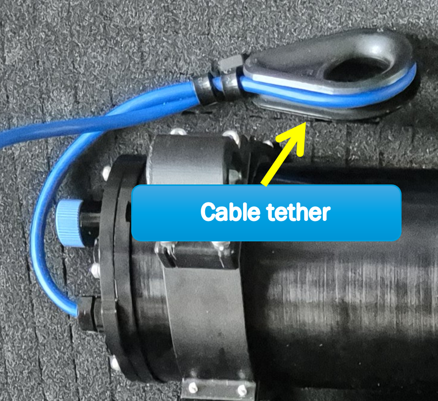
- Wrap the section of the cable that is close to the device around the provided cable tether and secure it with tie-wraps, as shown in Figure 1. Then, tie the cable tether to the rope holder (shown in Figure 2), to prevent mechanical stress on the device's cable.
- Secure the device to a rigid, non-ferromagnetic mounting frame. If the device is used without a mounting frame, pass a rope through both the rope holder and the cable tether to secure it.
- Connect the A and B RS485 wires to the A and B terminals of your RS485 communication device.
- Connect +V and the two GND wires to a DC power supply (7–30 VDC, ≥1 A). A 12 VDC power supply with minimal noise is recommended.
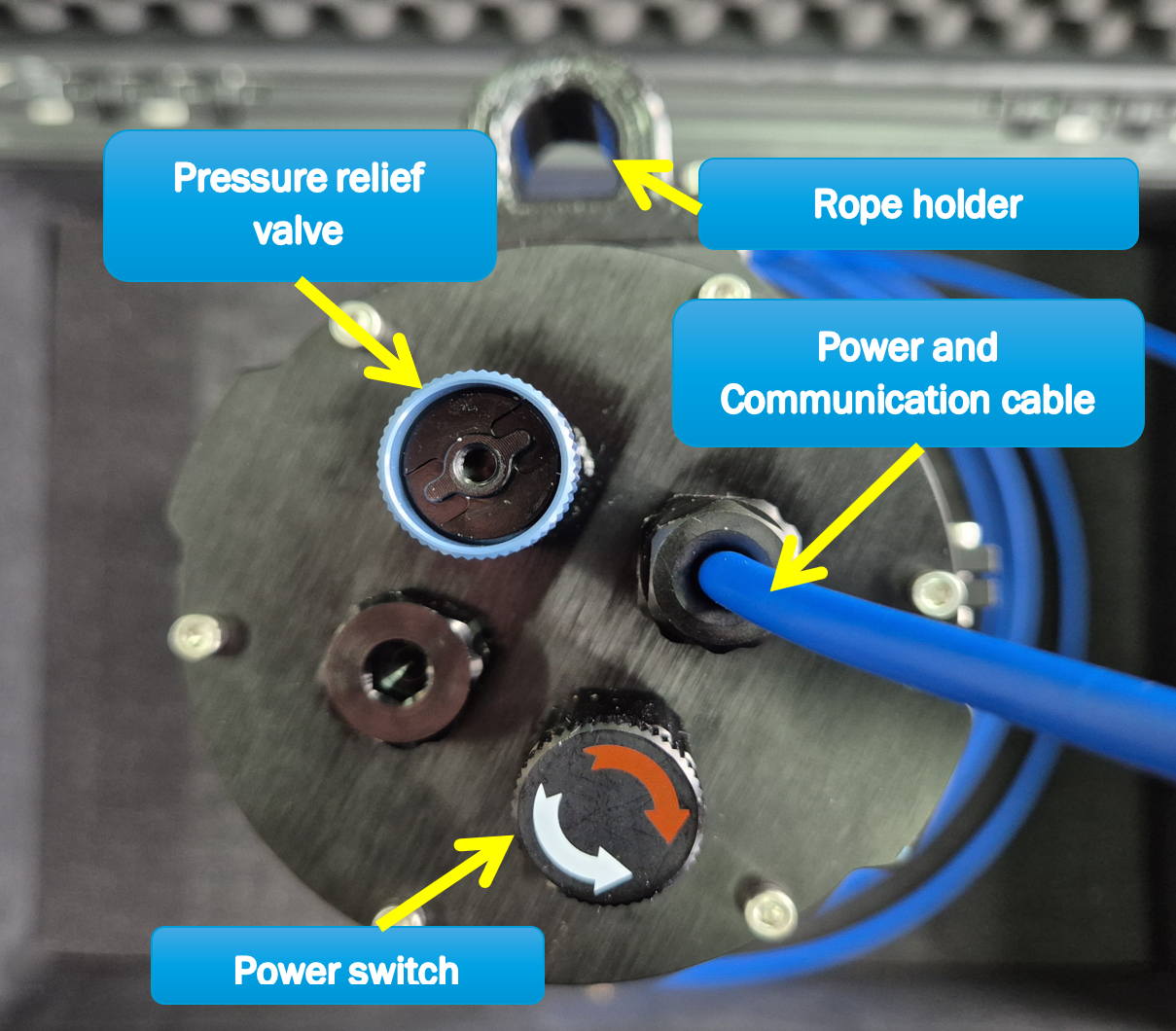
- Check that the pressure relief valve (shown in Figure 2) is placed on the device and is fully tightened. If not, tighten it by rotating it clockwise by hand.
- Power on the supply and verify that the voltage output is 7–30 VDC.
- Power on the device by rotating the ON/OFF circular Power switch (shown in Figure 2) clockwise by hand.
- Verify the data stream is consistent at your terminal device.
- Deploy to a depth of up to 50 m. Ensure data keeps updating and IMU (yaw, pitch, roll) values indicate no device motion (which would affect the magnetic measurements). Otherwise, reposition the device and/or use a more rigid mounting frame.
⚠ WARNING: Although the device includes reverse polarity protection, do not connect power terminals in reverse.
Wire Connections:
| Wire Color | Function |
|---|---|
| Silver | GND (Cable shielding) |
| Black | GND |
| Red | V+ (7–30 VDC) |
| White | RS485 A+ |
| Green | RS485 B- |
⚠ CAUTION: If the pressure relief valve is not fully tightened, the device will be flooded and permanently damaged!
3.2 Upon Retrieval
- Turn the ON/OFF circular switch counterclockwise to power off the device.
- Disconnect the device wires from the power supply and RS485 communication device.
- Clean the device and its cable with fresh water and mild dish soap.
3.3 Transportation and Storage
⚠ CAUTION: When transported by air, both the device’s and the case’s pressure relief valves must be loosened to prevent pressure-related issues.
- Avoid shocks, impacts, or intense vibrations during transportation.
- Store the device in a dry environment at room temperature, away from flammable materials and strong magnetic fields.
4. RS-485 Communication
4.1 Connecting to the Device
The device uses Modbus RTU over RS-485.
Connection settings:
| Setting | Value |
|---|---|
| Baud rate | 115200 bps |
| Data bits | 8 |
| Parity | None |
| Stop bits | 1 |
4.2 Reading Acoustic Sensor Data (Slave ID = 1)
| Setting | Value |
|---|---|
| Modbus Slave ID | 1 |
| Modbus Function | 0x03 (Read Holding Registers) |
| Starting Address | 0 |
| Ending Address | 39 |
| Registers | Content | Unit | Type |
|---|---|---|---|
0–1 |
Frequency #1 | Hz | Float (IEEE 754) |
2–3 |
SPL #1 | dB re 1μPa | Float (IEEE 754) |
4–5 |
Frequency #2 | Hz | Float (IEEE 754) |
6–7 |
SPL #2 | dB re 1μPa | Float (IEEE 754) |
| ... pattern repeats for #3 through #9 ... | |||
36–37 |
Frequency #10 | Hz | Float (IEEE 754) |
38–39 |
SPL #10 | dB re 1μPa | Float (IEEE 754) |
4.3 Reading Magnetic Sensor Data (Slave ID = 2)
| Setting | Value |
|---|---|
| Modbus Slave ID | 2 |
| Modbus Function | 0x03 (Read Holding Registers) |
| Starting Address | 0 |
| Ending Address | 9 |
| Registers | Content | Unit | Type |
|---|---|---|---|
0–1 |
X-axis magnetic field | nT | Float (IEEE 754) |
2–3 |
Y-axis magnetic field | nT | Float (IEEE 754) |
4–5 |
Z-axis magnetic field | nT | Float (IEEE 754) |
6–7 |
Total magnitude | nT | Float (IEEE 754) |
8–9 |
Deviation | nT | Float (IEEE 754) |
Temperature Compensation (optional)
The slave can apply a per-axis linear correction to the decimated magnetic stream to remove the fluxgate's offset-vs-temperature drift before it reaches the slow-median, DC-variation, and Total field outputs:
x_corrected = x_dec + βx · (T − T0)Coefficients are entered from the dashboard's Temperature Compensation card (Device tab) or via Modbus / MQTT. They are persisted in the slave's NVS and survive reboots. The correction is inert by default (β = 0, valid flag = 0) and applied only after at least one β has been set; clearing the coefficients restores the uncorrected stream. The live anomaly-detection path (X/Y/Z filtered) is intentionally untouched, since its rolling baseline already absorbs slow thermal drift.
| Registers | Content | Unit | Type |
|---|---|---|---|
99–100 |
βx (read-back) | nT / °C | Float (IEEE 754) |
101–102 |
βy (read-back) | nT / °C | Float (IEEE 754) |
103–104 |
βz (read-back) | nT / °C | Float (IEEE 754) |
105–106 |
T0 reference temperature (read-back) | °C | Float (IEEE 754) |
107 |
Compensation valid flag (1 = active, 0 = inert) | — | uint16 |
To set a coefficient, write the corresponding command code and an
IEEE-754 float value to the MAD command registers (40–42): code 40
sets βx, 41 sets βy, 42 sets βz,
43 sets T0, and 44 clears all β and disables the
correction. Setting any β automatically asserts the valid flag.
4.4 Reading Environmental Sensor Data (Slave ID = 2)
| Setting | Value |
|---|---|
| Modbus Slave ID | 2 |
| Modbus Function | 0x03 (Read Holding Registers) |
| Starting Address | 11 |
| Ending Address | 16 |
| Registers | Content | Unit | Type |
|---|---|---|---|
11–12 |
Temperature | °C | Float (IEEE 754) |
13–14 |
Humidity | %RH | Float (IEEE 754) |
15–16 |
Pressure | hPa | Float (IEEE 754) |
4.5 Reading IMU Data (Slave ID = 2)
| Setting | Value |
|---|---|
| Modbus Slave ID | 2 |
| Modbus Function | 0x03 (Read Holding Registers) |
| Starting Address | 17 |
| Ending Address | 22 |
| Registers | Content | Unit | Type |
|---|---|---|---|
17–18 |
Yaw | degrees | Float (IEEE 754) |
19–20 |
Pitch | degrees | Float (IEEE 754) |
21–22 |
Roll | degrees | Float (IEEE 754) |
4.6 Data Decoding
All sensor data are encoded as 32-bit IEEE 754 floating-point numbers, split across two consecutive 16-bit holding registers.
Register layout:
- First register (lower address): bits 0–15 of the 32-bit float (low word)
- Second register (higher address): bits 16–31 of the 32-bit float (high word)
Example: Reading registers 0–1 of Slave ID = 1, with values
0x0000 and 0x447A:
uint32 = (0x447A << 16) | 0x0000 = 0x447A0000
# IEEE 754 → 1000.0 (Hz)
Python snippet:
import struct
raw = (0x447A << 16) | 0x0000
value = struct.unpack('f', struct.pack('I', raw))[0]
Full example code — download rs485_example.py
# pip install pymodbus pyserial

import struct
import time
import sys
from pymodbus.client import ModbusSerialClient

CURSOR_HOME = "\033[H"
CLEAR_SCREEN = "\033[2J"
CLEAR_TO_END = "\033[J"

COM_PORT = "COM16"  # Change to your port (e.g. /dev/ttyUSB0 on Linux)
BAUD_RATE = 115200
POLL_INTERVAL = 0.2  # seconds

def decode_float(low, high):
    raw = (high << 16) | low
    return struct.unpack('f', struct.pack('I', raw))[0]

def read_acoustic(client, lines):
    try:
        result = client.read_holding_registers(0, count=40, device_id=1)
        if result.isError():
            lines.append(f"  Acoustic read error ({result})")
            return
        regs = result.registers
    except Exception as e:
        lines.append(f"  Acoustic offline ({e})")
        return

    lines.append("  Acoustic — Top Frequencies:")
    for i in range(10):
        base = i * 4
        freq = decode_float(regs[base], regs[base + 1])
        spl = decode_float(regs[base + 2], regs[base + 3])
        lines.append(f"    #{i+1:2d}  {freq:10.2f} Hz  {spl:8.2f} dB")

def read_magnetic(client, lines):
    try:
        result = client.read_holding_registers(0, count=37, device_id=2)
        if result.isError():
            lines.append(f"  Magnetic read error ({result})")
            return
        regs = result.registers
    except Exception as e:
        lines.append(f"  Magnetic offline ({e})")
        return

    lines.append("  Magnetic Field:")
    lines.append(f"    X: {decode_float(regs[0], regs[1]):.2f} nT")
    lines.append(f"    Y: {decode_float(regs[2], regs[3]):.2f} nT")
    lines.append(f"    Z: {decode_float(regs[4], regs[5]):.2f} nT")
    lines.append(f"    Total: {decode_float(regs[6], regs[7]):.2f} nT")
    lines.append(f"    Deviation: {decode_float(regs[8], regs[9]):.2f}")

    lines.append("  Environment:")
    lines.append(f"    Temperature: {decode_float(regs[11], regs[12]):.2f} °C")
    lines.append(f"    Humidity: {decode_float(regs[13], regs[14]):.2f} %RH")
    lines.append(f"    Pressure: {decode_float(regs[15], regs[16]):.2f} hPa")

    lines.append("  Orientation:")
    lines.append(f"    Yaw: {decode_float(regs[17], regs[18]):.2f}°")
    lines.append(f"    Pitch: {decode_float(regs[19], regs[20]):.2f}°")
    lines.append(f"    Roll: {decode_float(regs[21], regs[22]):.2f}°")

def main():
    client = ModbusSerialClient(
        port=COM_PORT, baudrate=BAUD_RATE,
        bytesize=8, parity='N', stopbits=1, timeout=1,
    )
    if not client.connect():
        print("Could not connect. Check COM port.")
        sys.exit(1)

    sys.stdout.write(CLEAR_SCREEN)
    print(f"Reading from {COM_PORT}. Press Ctrl+C to stop.\n")
    try:
        while True:
            lines = []
            now = time.time()
            ms = int((now % 1) * 1000)
            lines.append(time.strftime("[%H:%M:%S", time.localtime(now)) + f".{ms:03d}]")
            read_acoustic(client, lines)
            read_magnetic(client, lines)
            sys.stdout.write(CURSOR_HOME + "\n".join(lines) + "\n" + CLEAR_TO_END)
            sys.stdout.flush()
            time.sleep(POLL_INTERVAL)
    except KeyboardInterrupt:
        print("\nStopped.")
    finally:
        client.close()

if __name__ == "__main__":
    main()
5. Acquired Data Examples
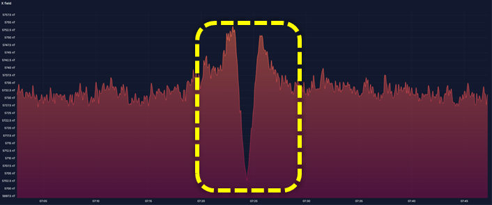
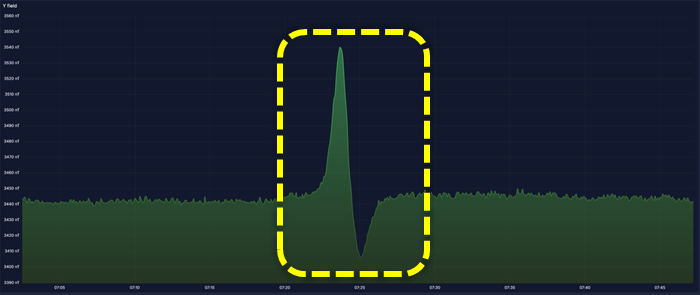
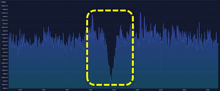
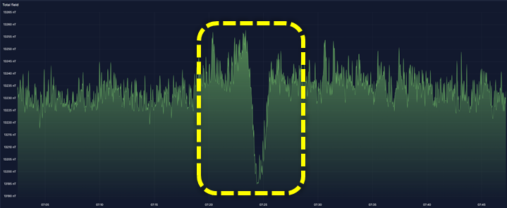
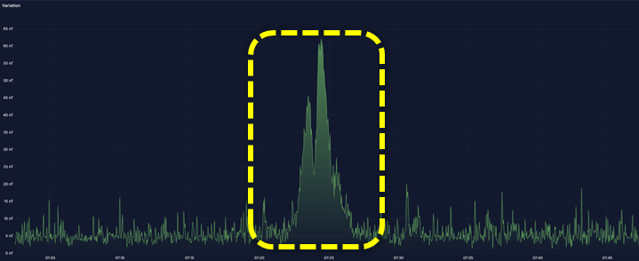
5.1 Magnetic Detection
In the following figures, the magnetic data retrieved during the detection of a ship are depicted. The magnetic field variation is easily observed at all 3 magnetometer axes, as well as at the total magnetic field plot. To distinguish it even better, the device uses a model to calculate the magnetic field deviation of recent readings from a rolling average baseline.
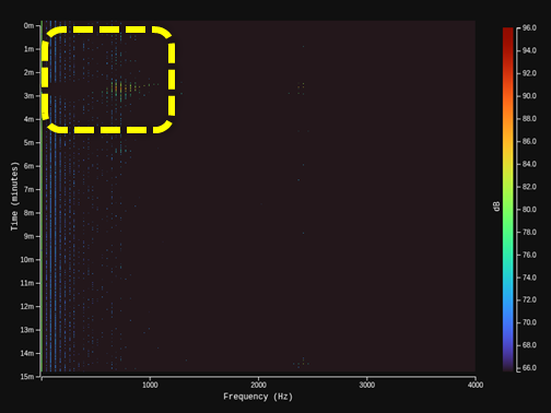
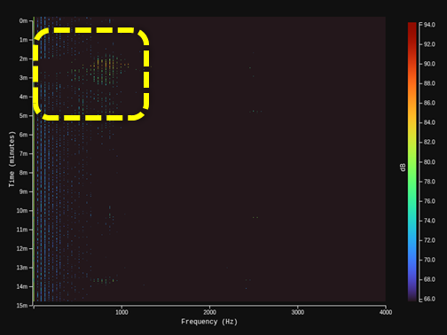
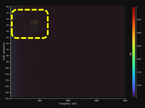
5.2 Acoustic Detection
In the following figures, the acoustic data captured during the detection of different ships are presented as spectrograms that include the 10 most dominant frequencies, calculated by the device implementing a Fast Fourier Transform (FFT).
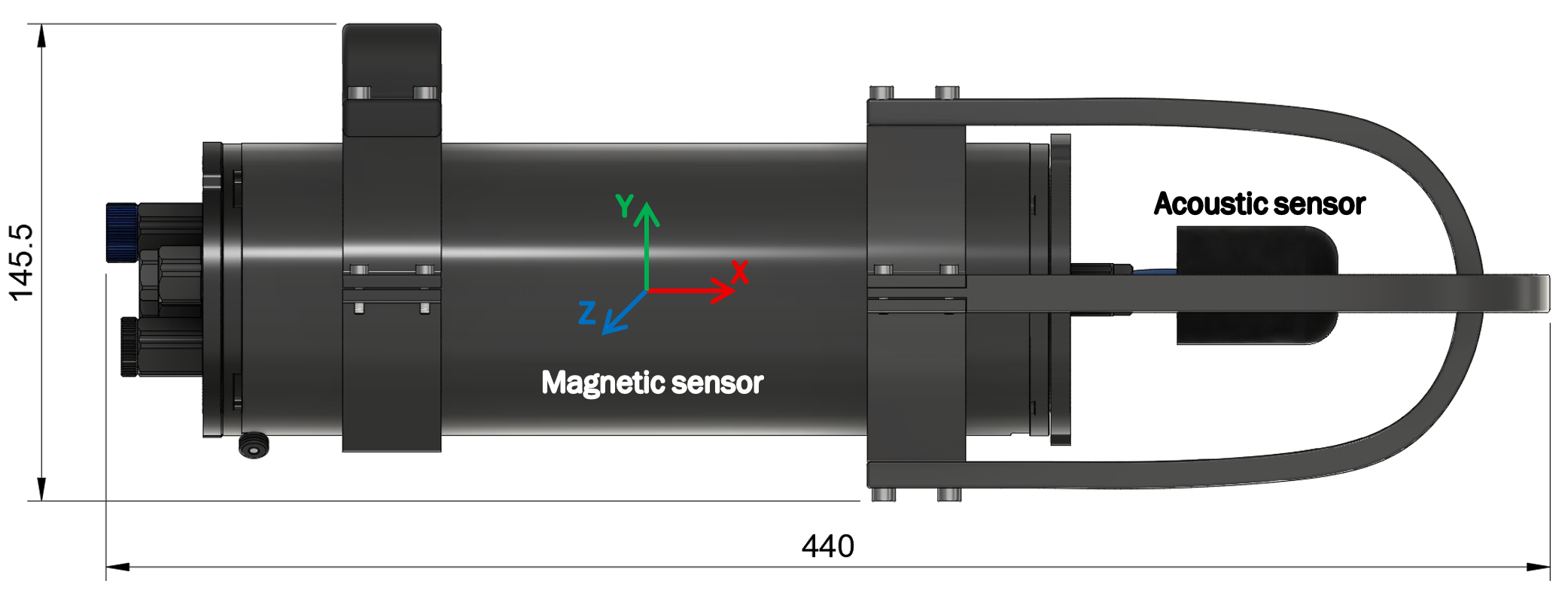
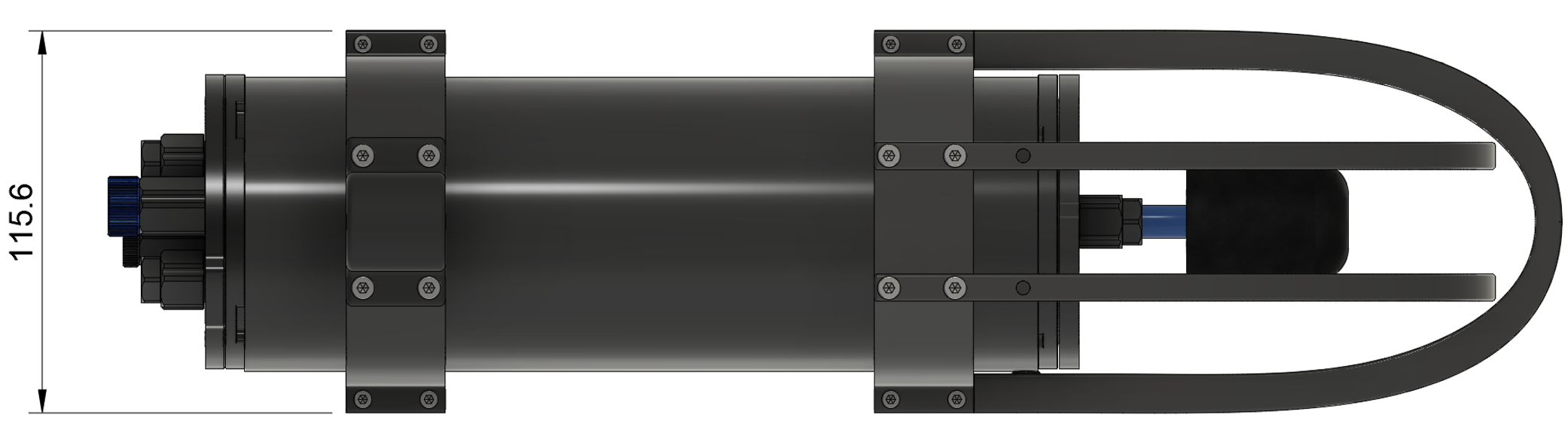
6. Device Dimensions
7. Technical Specifications
| Parameter | Value |
|---|---|
| Power | |
| Supply voltage | 7–30 VDC |
| Supply current | ~200 mA at 12 VDC |
| Power consumption | 2.5 W |
| Communication | |
| Output | Digital |
| Interface | RS485 |
| Protocol | Modbus RTU |
| Baud rate | 115200 bps |
| Typical polling rate | 1–10 Hz |
| Enclosure | |
| Material | Anodized aluminum |
| Diameter | 145.5 mm |
| Length | 440 mm |
| Operating temperature | -10°C to +80°C |
| Recommended depth | 50 m |
| Maximum depth | 300 m |
| Weight (in air) | 1900 g |
| Cable | |
| Length | 3 m |
| Outer diameter | 5.3 mm |
| Weight (in air) | ~138 g |
| Structure | 2 shielded twisted pairs |
| Wire size | 22 AWG |
| Jacket | LSZH (Low Smoke Zero Halogen) |
| Operating temperature | -20°C to 80°C |
| Magnetic Sensor | |
| Noise level | <15 pT/√Hz |
| Sensitivity | 97 mV/μT |
| Absolute range | 65 μT |
| Frequency response | DC to 10 Hz |
| Acoustic Sensor | |
| Sensitivity | -190 dB re 1 V/μPa |
| Bandwidth | 10 Hz to 50 kHz |
| Sensing element | PZT (Lead Zirconate Titanate) |
| Encapsulation | Polyurethane resin |
| IMU | |
| Pitch accuracy | ~1° |
| Roll accuracy | ~1° |
| Yaw accuracy | ~2–5° |
| Temperature Sensor | |
| Range | -40°C to +85°C |
| Accuracy | ±1°C |
| Resolution | ~0.01°C |
| Humidity Sensor | |
| Range | 0–100% RH |
| Accuracy | ±3% RH |
| Resolution | ~0.008% RH |
| Pressure Sensor | |
| Range | 300–1100 hPa |
| Accuracy | ±1 hPa |
| Resolution | ~0.18 Pa |
8. Troubleshooting
| Symptom | Possible Cause | Solution |
|---|---|---|
| No response from both nodes | Device not powered | Check power supply wiring; ensure power switch is fully turned clockwise |
| No response from both nodes | A/B wires swapped | Swap A and B connections on the adapter |
| No response from both nodes | Wrong COM port | Check Device Manager (Windows) or ls /dev/ttyUSB* (Linux) |
| No response from both nodes | Baud rate mismatch | Ensure baud rate is set to 115200 |
| No response from both nodes | GND not connected | Ensure adapter and device share the same GND |
| No response from one node | Wrong slave ID | Acoustic = 1, Magnetic/IMU/Env = 2 |
| Intermittent timeouts | Electrical noise | Relocate the cable away from sources of electrical noise |
| Data lag or corrupted | Polling rate outside the typical range | Set polling between 1–10 Hz. If still unstable, start at 1 Hz and increase gradually. |
| Data reads 0 or NaN | Sensor hardware fault | Power cycle the device (OFF then ON) |
| Magnetic saturated / not changing | Strong magnetic field | Relocate the device and/or check for nearby magnets or ferromagnetic objects |
| Magnetic fluctuates a lot | Motion artifacts | Stabilize the device |
| Acoustic not changing | Hydrophone obstructed | Ensure hydrophone is unobstructed and fully submerged |
9. Compliance & Disposal
EMC Notes: The device is intended for underwater use only and does not emit RF. Under 50 Hz magnetic field exposure, magnetic measurements may deviate up to 5%. Under 150–300 MHz RF exposure, deviation may reach 100%.
Export Control: Does not meet dual-use criteria. No export license required.
CE Compliance: Complies with applicable EU directives. Declaration of Conformity available on request.
RoHS Compliance: Complies with RoHS Directive 2011/65/EU and amendments. PZT hydrophone contains lead under applicable exemption.
Disposal: Contains electronic components. Do not dispose with household waste. Contact your local waste authority for recycling options.